Generates grade of membership, “admixture”, “topic” or “Latent Dirichlet Allocation” models, by representing sampling units as partial memberships in multiple groups. It can group regions based on phylogenetic information or functional traits.
fitgom(
  x,
  trait = NULL,
  cut = NULL,
  phy = NULL,
  bin = 10,
  na.rm = FALSE,
  K,
  shape = NULL,
  initopics = NULL,
  tol = 0.1,
  bf = TRUE,
  kill = 2,
  ord = TRUE,
  verb = 1,
  ...
)
Arguments
- x
A community data in long format with one column representing sites labeled “grids” and another column representing species labeled “species”.
- trait
A data frame or matrix object with the first column labeled “species” containing the taxonomic groups to be evaluated whereas the remaining columns have the various functional traits. The variables must be a mix of numeric and categorical values.
- cut
The slice time for the phylogenetic tree.
- phy
is a dated phylogenetic tree with branch lengths stored as a phylo object (as in the ape package).
- bin
The desired number of clusters or bins.
- na.rm
Logical, whether NA values should be removed or not.
- K
The number of latent topics. If length(K)>1, topics will find the Bayes factor (vs a null single topic model) for each element and return parameter estimates for the highest probability K.
- shape
Optional argument to specify the Dirichlet prior concentration parameter as shape for topic-phrase probabilities. Defaults to 1/(K*ncol(counts)). For fixed single K, this can also be a ncol(counts) by K matrix of unique shapes for each topic element.
- initopics
Optional start-location for \([\theta_1, \ldots, \theta_K]\), the topic-phrase probabilities. Dimensions must accord with the smallest element of K. If NULL, the initial estimates are built by incrementally adding topics.
- tol
An indicator for whether or not to calculate the Bayes factor for univariate K. If length(K)>1, this is ignored and Bayes factors are always calculated.
- bf
An indicator for whether or not to calculate the Bayes factor for univariate K. If length(K)>1, this is ignored and Bayes factors are always calculated.
- kill
For choosing from multiple K numbers of topics (evaluated in increasing order), the search will stop after kill consecutive drops in the corresponding Bayes factor. Specify kill=0 if you want Bayes factors for all elements of K.
- ord
If
TRUE, the returned topics (columns of theta) will be ordered by decreasing usage (i.e., by decreasingcolSums(omega)).- verb
A switch for controlling printed output. verb > 0 will print something, with the level of detail increasing with verb.
- ...
Further arguments passed to or from other methods.
Value
An topics object list with entries
KThe number of latent topics estimated. If inputlength(K)>1, on output this is a single value corresponding to the model with the highest Bayes factor.thetaThe ncolcounts by K matrix of estimated topic-phrase probabilities.omegaThe nrowcounts by K matrix of estimated document-topic weights.BFThe log Bayes factor for each number of topics in the input K, against a null single topic model.DResidual dispersion: for each element of K, estimated dispersion parameter (which should be near one for the multinomial), degrees of freedom, and p-value for a test of whether the true dispersion is >1.XThe input community matrix as a sparse matrix.
Details
Mapping phylogenetic regions (phyloregions) involves successively slicing the phylogenetic tree at various time depths (e.g., from 1, 2, 3, 4, to 5 million years ago (Ma)), collapsing nodes and ranges that originated at each time depth, and generating a new community matrix based on the presence or absence of each lineage in a grid cell. A grade of membership model is then fitted to the reduced community matrix. To map functional trait regions (traitregions), the function uses k-means to cluster species based on their functional traits, often for mixed-type data including categorical and numeric functional traits. The ranges for each species in each resulting cluster are collapsed to generate a new community matrix based on the presence or absence of cluster representative in a grid cell. A grade of membership model is then fitted to the new reduced community matrix. Mapping bioregions for taxonomic diversity is based on fitting a grade of membership model directly to the original community matrix that is often represented with species in the columns and sites as rows.
Examples
library(terra)
data(africa)
names(africa)
#> [1] "comm" "phylo" "mat" "IUCN" "K" "theta" "omega" "trait"
p <- vect(system.file("ex/sa.json", package = "phyloregion"))
m <- fitgom(x=sparse2long(africa$comm), K=3)
#>
#> Estimating on a 365 document collection.
#> Fit and Bayes Factor Estimation for K = 3
#> log posterior increase: 2320.8, 347.5, 90.9, 67.6, 96.4, 24.7, 2.5, 0.3, 0.1, done.
#> log BF( 3 ) = 20904.81
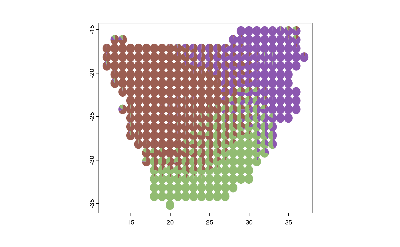
COLRS <- phyloregion:::hue(m$K)
plot_pie(m$omega, pol = p, col=COLRS)